Skip to content

Mortality & longevity

Mortality: Good things come to those who weight (II)

Maths!

This article is almost all maths.

If that’s not your thing then I suggest that you skip ahead to part III (to come).

In the previous article, I noted that the the ultimate objective when assessing base pensioner mortality for DB plans is to determine the present value of the liabilities, as opposed to selecting and calibrating an abstract model.

In this article, I’ll use a simple framework to express this mathematically.

Mortality: Good things come to those who weight (I)

There was a time when actuaries understood that amounts-weighted statistics are the most appropriate ones for assessing DB pension plan liabilities. After all,

  • the objective is to value liabilities,
  • liability is proportional to pension amount, and
  • pension amount is a strong predictor of mortality,

and so weighting the experience data by what actually matters seems sensible.

Distribution of individuals (‘lives-weighted’) Concentration
Distribution of pension amount (‘amounts-weighted’) Concentration

But then some actuaries noticed that statistics textbooks do not mention weighting by amounts, and so they decided that it must be wrong.

Mortality: Pensioner mortality variation

Modelling the mortality of DB pensioners is, in many ways, about as easy as mortality modelling gets – experience data is typically very high quality and often strongly credible, anti-selection is not usually a big deal and the available rating factors are limited (which constrains model complexity).

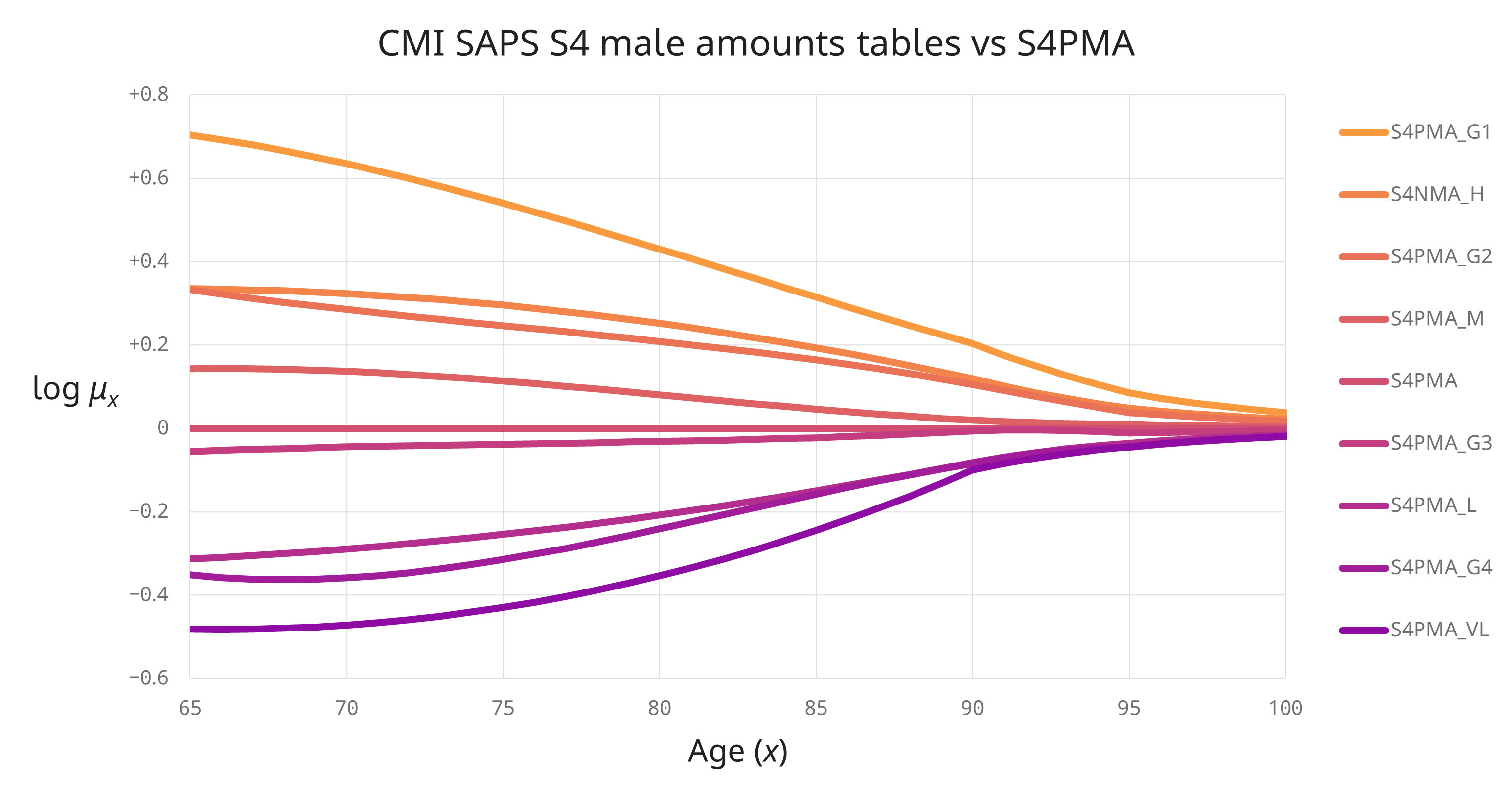
I suggest that it’s even simpler in that, for most pension plan mortality modelling, it is sufficient to assume that pensioner mortality varies monotonically in one-dimension along a low-high mortality axis.

Don’t just take my word for it; here’s how log mortality varies for the CMI’s S4 male pensioner base tables:

CMI SAPS S4 male amounts tables vs S4PMA CMI SAPS S4 male amounts tables vs S4PMA

Mortality: Incoherent rating factors

A pre-requisite for pension plan mortality modelling is that the rating factors used should be coherent, which I’ll define shortly.

The insidious problem with incoherent rating factors is that a model may produce poor or even systemically biased forecasts while simultaneously performing well on standard model fit and selection diagnostics. Yikes!

For large experience datasets in particular, rating factor incoherence can be a bigger issue than model fitting and selection. But too often in practice, I’ve seen this issue trivialised or deemed ‘obvious’.

Mortality: Suddenly AIC

In this article, I’m going to look at choosing between mortality models using Hirotugu Akaike’s information criterion, the AIC.

I’m going to run through – at a very high level – the rationale behind the AIC and its construction because

  • the standard result looks so trivial that people sometimes assumes it’s an arbitrary convention, and
  • I’m going to generalise it (a little).

Mortality: Proportional hazards

A/E diagnostics are important but, if we have any mortality experience data, we should be using it to develop a model that takes account of that data, even if it’s nothing more than a simple how-much-heavier-or-lighter-is-the-mortality-of-this-population-than-average model. Otherwise, we’re not making full use of available information.

There are lots of possible approaches, including complex parametric formulas designed to capture all typically observed effects. But I promised concision and so in this article I’ll expound what I think is simultaneously one of the most powerful general approaches and one of the simplest. And the beauty of it is: we’ve already done most of the work.

Mortality: Log-likelihood

I think it’s a shame that the ‘log’ in ‘log-likelihood’ is so often presented as a technical convenience or a device for avoiding numerical under/overflow. Yes, it is definitely both of these things, but it is much more fundamental.

Expected log-probability, i.e. entropy, lies at the heart of information theory. And the concept of entropy itself is pervasive, having extended beyond thermodynamics, its original home, into quantum physics and general relativity, as well as information theory.

So, without further ado, let’s define log-likelihood for mortality experience data.

Mortality: A over E

Why ‘A over E’?

‘A over E’ literally refers to ‘actual’ deaths divided by ‘expected’ deaths as a measure of how experience data compares with a mortality.

In practice, ‘A over E’ is often interpreted as meaning the whole statistical caboodle, which is how I’ll use it here.

In the previous article we defined experience data, variables and mortality with respect to that data, and the \(\text{A}\) (actual) and \(\text{E}\) (expected) deaths operators.

In this article we’ll put \(\text{A}\) and \(\text{E}\) to work.

Mortality: Measures matter

This is the first in a series of articles outlining mortality experience analysis fundamentals, by which I mean estimating the underlying mortality for individuals in a defined group (e.g. members of a pension plan) from mortality experience data.

This will be fairly technical, but I’ll aim

  • to be concise,
  • to pull out the key insights, including what does and doesn’t matter in practice, and
  • to map concepts one-to-one to the process of actually carrying out a mortality experience analysis or calibrating and selecting mortality models.